Kratos MDPA Preview (VS Code extension)
     
📖 Read the full documentation »
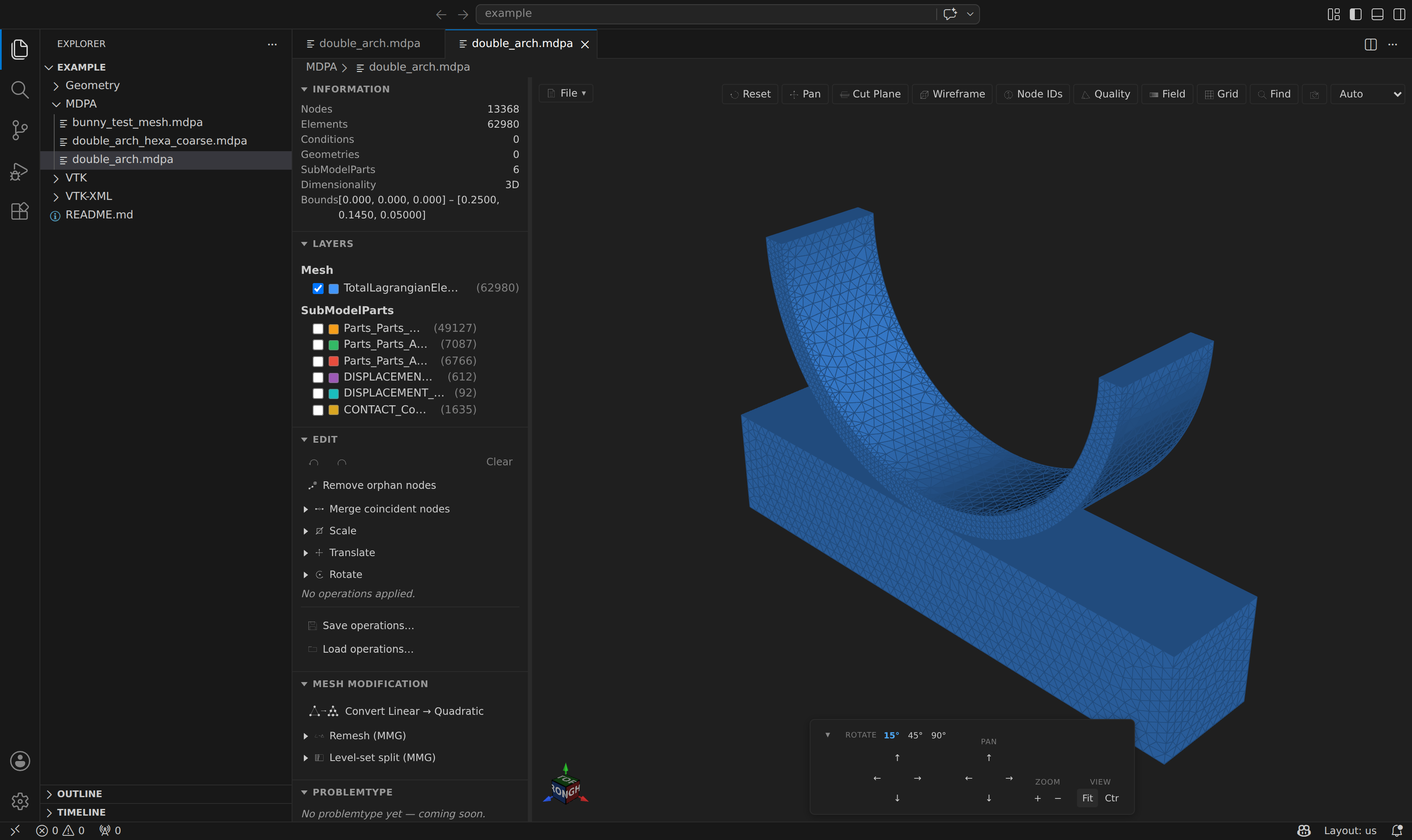
Preview, organize, edit, and remesh Kratos Multiphysics .mdpa model-part files directly in VS Code: a 3D mesh viewer with a navigable ModelPart / SubModelPart outline whose entries are toggleable layers.
It is fully self-contained — a pure-TypeScript parser feeds a VTK.js viewer running in a webview. No Python or compiled Kratos is required.
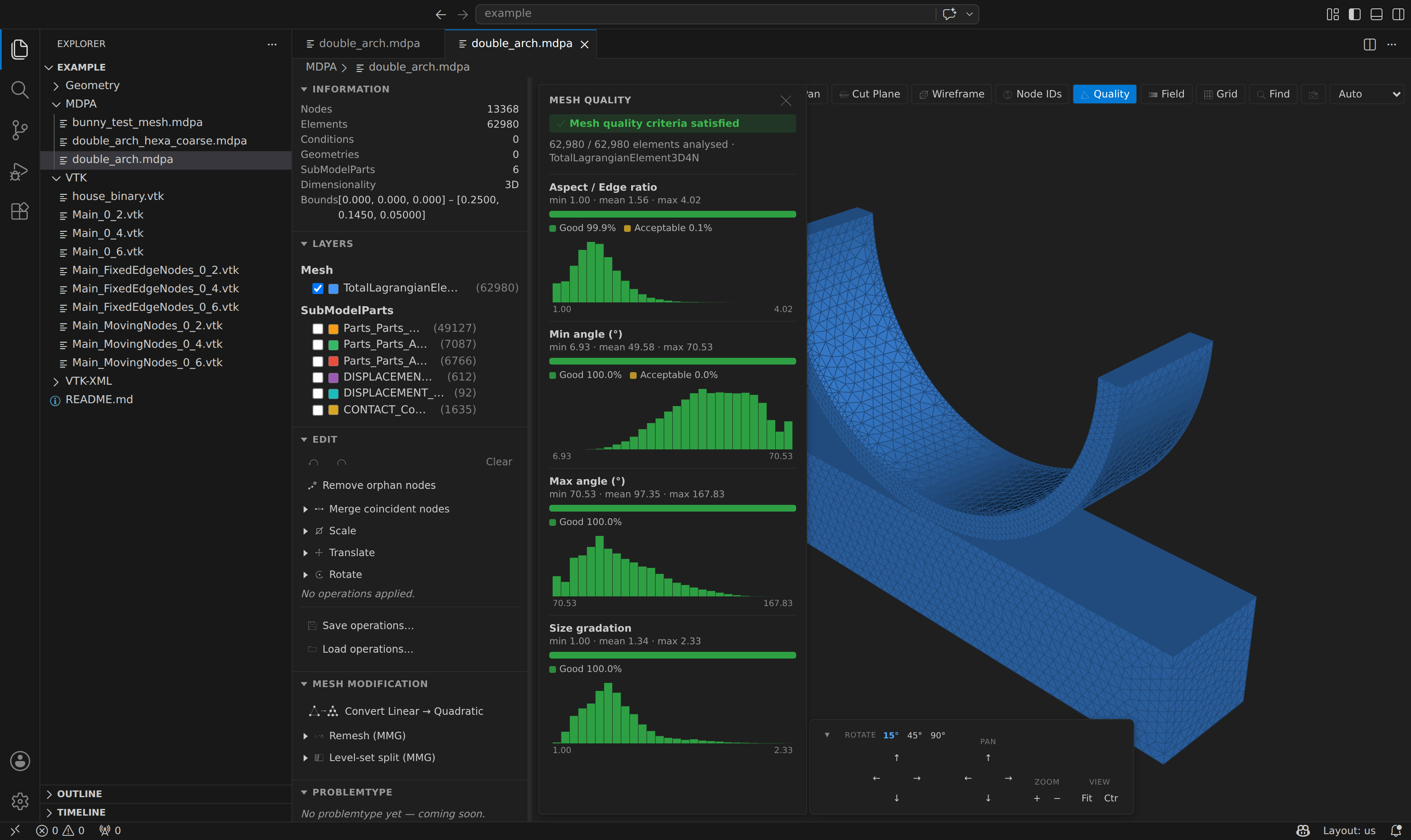
| Mesh quality |
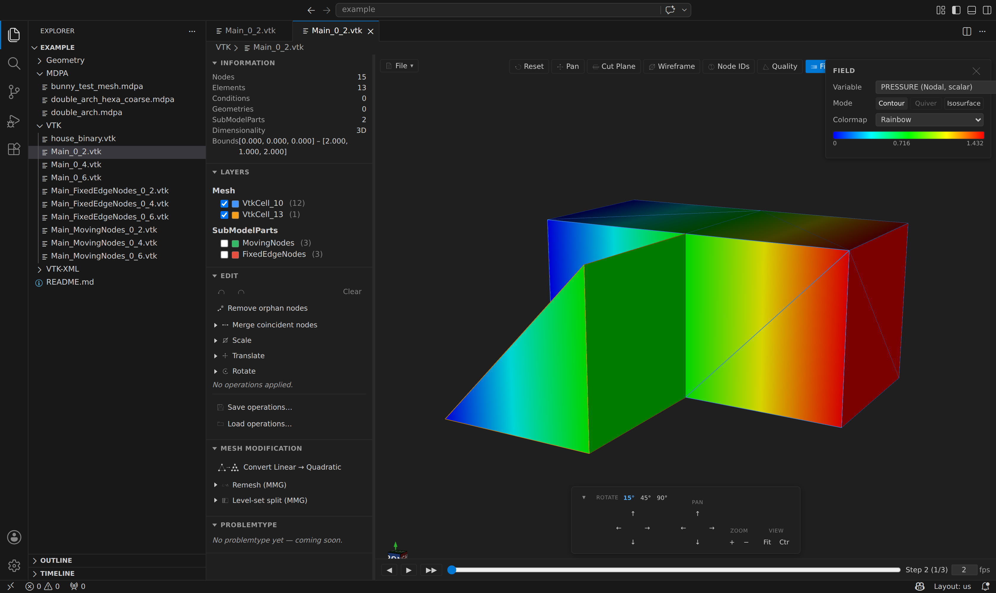
Field contour |
 |
 |
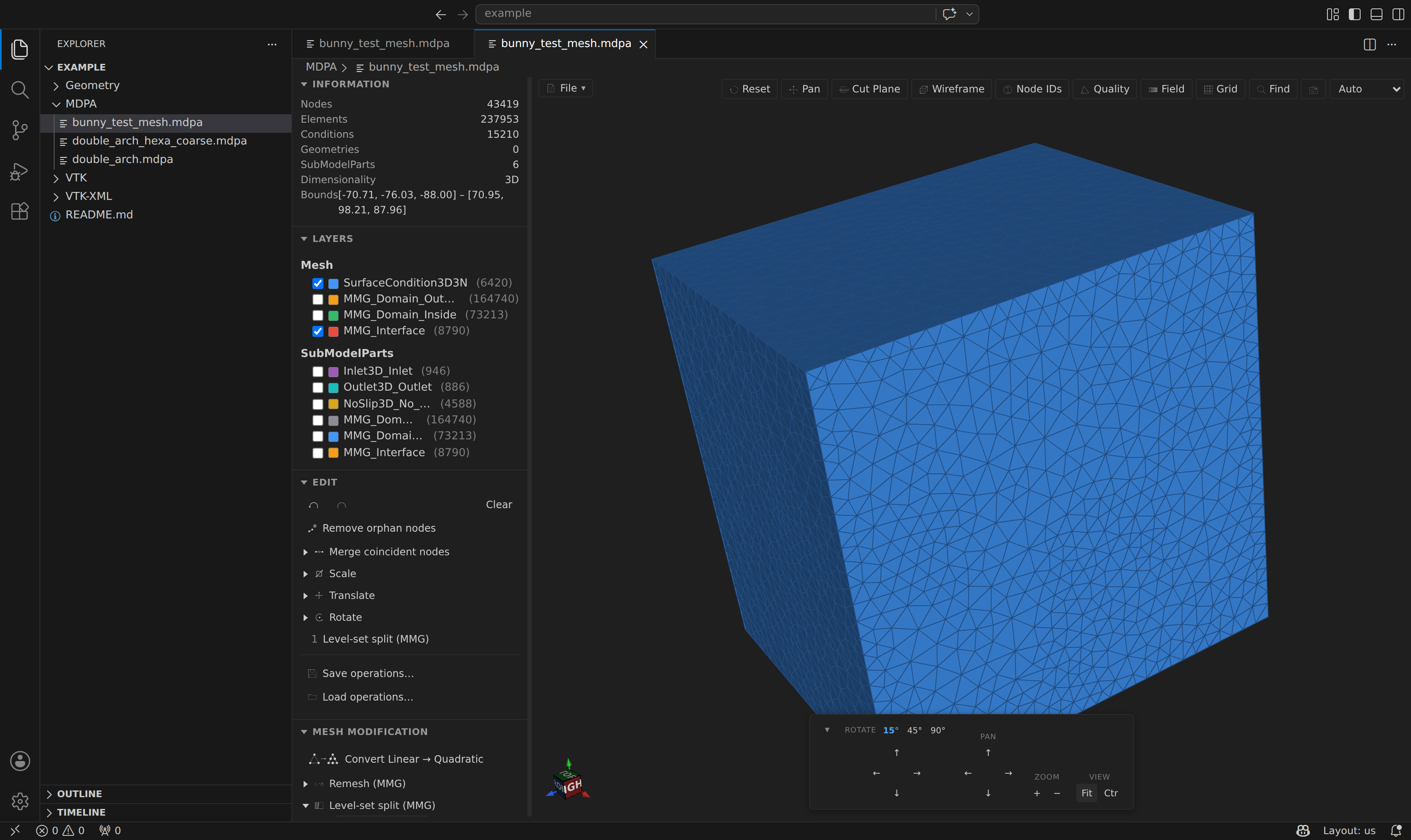
| Level-set split (MMG) |
Linear → Quadratic |
 |
 |
| Problemtype: build & run Kratos cases |
Sphere / particle elements (Advanced menu) |
 |
 |
| Additional mesh operations |
Face normals (Advanced menu) |
 |
 |
📖 See the full documentation for a screenshot-rich walkthrough of every feature.
Features
Open it from the sidebar, with no file open. A Kratos icon in VS Code's activity bar opens a panel offering Open Mesh File…, Open Empty Preview (the viewer itself, over an empty viewport) and Load Problem…, plus a Recent Meshes list of the last ten meshes you opened. Tracked solver runs (Kratos Runs) show up there too, alongside their usual place in the Explorer.
Read and write OpenFOAM cases. Open a case's .foam marker and its constant/polyMesh/ is loaded, with each boundary patch as a named SubModelPart (inlet, outlet, …) so boundary conditions can be assigned to it. Compressed (writeCompression on) cases are decompressed automatically, and the preview watches constant/polyMesh/ so re-running blockMesh refreshes it in place. Saving in place is refused — the marker is an empty file and the mesh is its siblings — so use Export or Save As to write a new case. See OpenFOAM Cases.
A header summary for a mesh too large to open. Above kratos.preview.summaryThresholdMb (default 250 MB, 0 disables it) the preview reports what is in the file — counts, entity blocks, variable names, regions, time steps — with one Open full mesh anyway button, instead of parsing a file that would hang the window. It works for every supported format, and says what the answer cost: a bounded header read for VTK XML, PLY, binary STL and .vtm; a single allocation-free stream for .mdpa, .obj and ASCII STL (.mdpa declares no counts, so it has no header to read); a whole read for the meshio++ formats. See Header Summary.
3D preview of nodes, elements, conditions, and geometries. Volume elements (tet/hex/wedge/pyramid) are shown as their boundary surface; quadratic elements are approximated by their corner nodes.
Outline tree of the entity blocks and the full SubModelPart hierarchy, with per-row visibility checkboxes (activate/deactivate a layer) and click-to-frame. Drag the divider between the sidebar and the 3D view to resize the sidebar.
Reorganize the SubModelPart tree — every SubModelPart row carries an organize button offering New child, Move under, Merge into and Edit membership (add/remove node, element, condition or geometry ids by a comma/range list, e.g. 1,2,5-10), beside the existing rename and delete. The parent/child subset rule Kratos requires is maintained, not merely checked: adding an entity to a part also adds it to every ancestor and removing one also removes it from every descendant, which is exactly what ModelPart::AddNode / RemoveNode do upstream — so the tree you build is always one Kratos loads. Each is an undoable operation in the history and reachable from mesh_transform.
SubModelParts as layers — each SubModelPart is an independently toggleable overlay so you can isolate inlets/outlets/boundaries.
Stats panel: node/element/condition/geometry counts, bounding box, detected 2D/3D, and any element type names that could not be mapped.
Mesh quality (Quality toolbar button / Compute Mesh Quality command): purely geometric metrics inspired by Kratos' ComputeMeshQualityProcess — aspect/edge ratio, min/max angle (dihedral for volume cells, interior corner angles for surface cells), and per-node size gradation. Results are shown in a panel with per-metric histograms, a Good/Acceptable/Bad/Unacceptable breakdown, and an overall verdict. Bad elements can be highlighted in red and framed in the 3D view.
Mesh size (Advanced ▸ Mesh Size): compute per-node and per-element size and inspect the distribution.
- Nodal size (
NODAL_H) — a faithful port of Kratos' FindNodalHProcess: for each node, the minimum distance to any other node that shares an element.
- Element size — the element characteristic length (mean edge length).
- Color the mesh field-like by either measure, and read a floating box-and-whisker plot of the element-size distribution. Highlight the smallest and largest elements (statistical IQR outliers) — small in blue, large in red — and frame them in the 3D view.
- Write to mesh appends
NODAL_H / ELEMENT_H to the mesh (an undoable operation) so they show in the Field panel and are saved with the file; the values are also cached for reuse by future operations.
Field visualization (Field toolbar button / Field Visualization command): plot the NodalData, ElementalData, and ConditionalData fields stored in the file. Pick a variable and switch on any combination of the five modes:
- Contour — color the mesh by a scalar (smooth point-data for nodal fields, flat per-cell for elemental/conditional). Vector fields default to magnitude, or pick a single X/Y/Z component.
- Quiver — arrow glyphs oriented and scaled by a vector field (at nodes, or at cell centroids for elemental/conditional data), colored by magnitude, with an adjustable arrow-scale slider.
- Isosurface — extract the surface where a scalar equals one or more slider-driven iso values (a count spinner adds evenly-spaced sliders; marching tetrahedra over volume cells, 2D / surface meshes fall back to iso-lines).
- Threshold — show only the Elements/Conditions whose value falls in an editable
[min, max] window; for nodal fields, choose whether a cell needs all or any of its nodes in range.
- Deformed shape — warp the geometry by a vector field × an adjustable scale (its own "Deform by" selector, independent of the coloring field), the canonical FE post-processing view. The deformation is global, so every other active mode renders on the deformed geometry.
Contour/Isosurface/Threshold share a color range that's editable and lockable (min/max inputs + reset-to-data button), an optional log scale, and discrete color banding (5/10/20 bands). A colormap dropdown (Rainbow/jet by default, plus Viridis, Plasma, Inferno, Magma, Cividis, Turbo, Cool-warm, Blue-Orange, Spectral, HSV, and Grayscale) drives the 3D coloring, a live panel legend, and an optional in-scene scalar bar that (unlike the panel legend) is captured by the Screenshot button; when the scalar bar is off, screenshots instead composite the legend onto the captured image.
Screenshot (View ▾ → Screenshot… / Screenshot to PNG… command / Ctrl+Alt+P): captures the current viewport as a PNG and opens a Save dialog pre-filled with the source file's name (e.g. mesh.png next to mesh.mdpa). Uses VTK.js's captureNextImage() for correct WebGL swap-chain timing. SVG export is not possible — the viewport is a rasterised WebGL canvas.
Find entity by ID (Find toolbar button / Find Entity by ID command): type a Node, Element, Condition, or Geometry ID to locate it instantly. The entity is highlighted in yellow and the camera zooms to it; all other layers switch to wireframe so the result stands out clearly. Closing the bar restores the previous display state.
Inspect (Inspect toolbar button): click any node, element, or condition on the mesh — no id needed up front, unlike Find — to see its id, block, SubModelPart membership, and every field value defined at it, in a floating panel. A Measure sub-mode inside the panel: click two nodes to draw a line between them and read the distance and Δx/Δy/Δz.
Run manager (Kratos Runs in the Explorer): running a case now tracks it. Live runs show elapsed time and the latest step written; finished ones show their exit code. Stop actually stops the solver, and results already written are kept. Runs survive the preview that started them.
Record a video (View ▾ ▸ Record…): capture the viewport as a WebM video or a numbered PNG sequence — either a playthrough of a mesh time series, or a camera turntable for a static mesh.
Split view (View ▾ ▸ Layout): show the mesh in 1, 2 or 4 viewports, each with its own camera, field settings and clip plane — DISPLACEMENT beside VELOCITY, or a clipped section beside the whole model. Orbit, pan and zoom act on whichever pane the pointer is in, and the focused pane (the one Reset/Frame, the Field panel and the Clip controls act on) is outlined.
Plot over time (Inspect panel, mesh previews with a time series): click a node or element, then Plot over time to chart one of its field values across every step of the series — one line per component, gaps where the value is missing rather than a line drawn through them. Click a point to jump the 3D view to that step, and export the series as CSV.
Data table (Advanced ▾ ▸ Data table…): the same values Inspect shows for one entity, for every entity at once — a scrollable table of nodes, elements, conditions or geometries with their coordinates or connectivity, optional SubModelPart membership, and every field defined there. Click a row to highlight and frame that entity in the scene; export the whole table as CSV or XLSX.
Clip (Clip toolbar button): an interactive clipping plane — pick the X / Y / Z axis or Free for an oblique cut (type a normal vector's X/Y/Z components), flip the direction, and drag the position slider — capped with a filled, field-colorable section and its element intersection edges rather than a hollow clip.
Layer opacity: hover any outline row for a small button that opens a live 0–100% opacity slider for that layer.
Rendering quality: the nav dock's ⋯ popover holds the scene-theme picker and a global model-opacity slider, and the dock itself a Persp/Ortho flip button that toggles perspective vs. orthographic camera projection; Lighting… exposes global specular / ambient / diffuse sliders and a backface-culling toggle; Camera Bookmarks… saves/restores named views for the session, with a JSON textarea for copying a view out or pasting one in. Standard axis views are one keypress away — 1–6 for ±X/±Y/±Z, i for an isometric corner.
Orientation cube + axis arrows — an always-visible labeled cube in the bottom-left corner of the viewport (RIGHT / LEFT / TOP / BOTTOM / FRONT / BACK) that follows the camera as you orbit. Prominent X (red), Y (green), and Z (blue) axis arrows with letter labels radiate from the cube. Clicking a face snaps the camera to that canonical axis direction.
Navigation dock — a floating one-row dock at the bottom-centre of the viewport that appears once a model loads (wraps to two rows in a narrow window; the chevron at its end collapses it):
- Reset view (default front view, framed), Fit (frames all visible geometry, same as the Reset Camera command), Zoom out / in (dolly ×0.8 / ×1.25; press-and-hold for continuous zoom).
- Shaded | Wire, the Clip group (Off/On, X/Y/Z/Free, position slider, live readout) and the Persp/Ortho flip.
- ⋯ popover (closes on an outside click or
Esc): Rotate compass with a 15°/45°/90° step picker, Pan compass (step proportional to the current zoom level), clip Flip and the Free-normal inputs, scene theme + model opacity, Edges, and Center (re-centers the focal point on the visible bounds without changing the orbit angle or zoom).
Background grid (View ▾ → Grid) — toggles a CubeAxesActor bounding box with labeled X/Y/Z axes and tick marks around the mesh. Colors adapt to the active scene theme.
Variables — the sidebar's named field registry, kept in sync with the Field panel (both list the same inventory; the panel badges fields that have a row, with a reveal jump). Every field on the mesh gets a row: file fields and computed ones alike. Add a variable by hand (+ Add variable), name it (e.g. d), pick how to compute it — a formula over coordinates and existing fields at any location (Nodal/Elemental/Conditional, like the Field calculator), the signed distance to a surface (an imported file, or a SubModelPart already in this mesh; same sign/band options as the Signed-distance form), any other Fields operation (average, gradient, Hessian, error estimate, transfer — same options as their forms, each with its form's icon), or a global reduction (min/max/minAbs/maxAbs/mean/std/median/sum/count/q1/q3/iqr of any field, e.g. maxAbs_TEMP; vectors reduce over magnitude) — then hit its own Play button. Computing a field from any Field form instead auto-creates the row for you, prefilled with that form's inputs. Once computed it is an ordinary field: the Field panel opens automatically, coloring the mesh by that variable, and it is immediately usable anywhere else a formula is accepted — the Field calculator, or the Remesh size = ƒ(h) formula — so d computed here can drive clamp(0.85*mean_h*(abs(d)/maxabs_d), 0.85*min_h, 1.15*max_h) in the Remesh form with no separate wiring. Variables combine freely: define one from a distance, then a second as a formula referencing the first, and so on. A row tracks the field it produced: if a timeline step replays without the async ops that computed it, the row says so and offers recompute instead of keeping a stale "Computed." — and if the computation itself produces nothing, the row reports the failure rather than hanging on "Computing…". Fields with no reconstructible definition (file fields and the like) render as locked rows — name, kind and origin, show-on-mesh, delete — and deleting any row removes only the row, never the field.
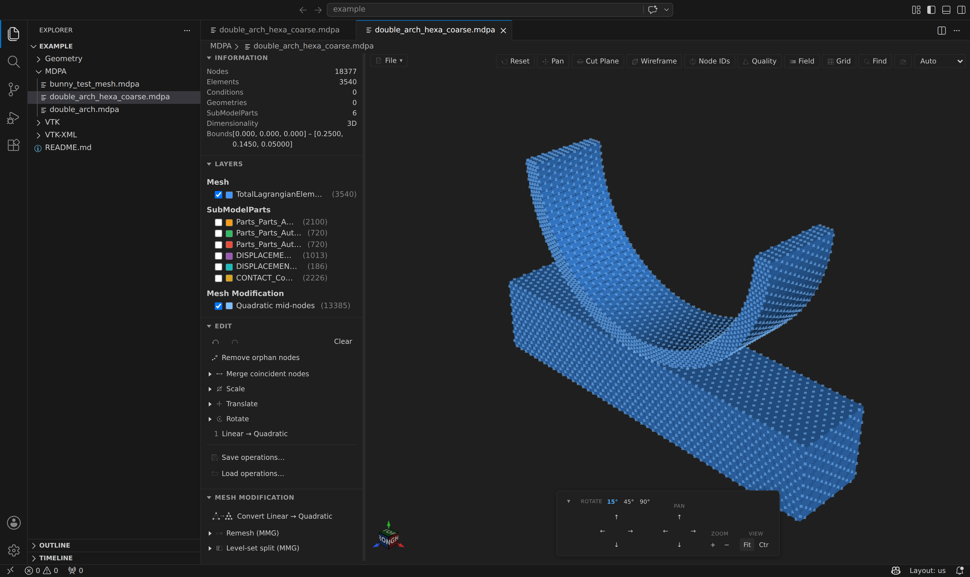
Mesh modification — the Mesh Modification sidebar section hosts in-place operations on the loaded mesh. Convert Linear → Quadratic inserts mid-edge nodes to raise every linear cell to its quadratic ("serendipity") counterpart — Triangle2D3→Triangle2D6, Quadrilateral2D4→Quadrilateral2D8, Tetrahedra3D4→ Tetrahedra3D10, Hexahedra3D8→Hexahedra3D20, Prism3D6→Prism3D15, Pyramid3D5→Pyramid3D13, Line2→Line3. Adjacent cells that share an edge get a single welded mid-edge node, nodal fields are interpolated at the new nodes, and SubModelParts are extended. The newly inserted mid-edge nodes are shown as a semitransparent Quadratic mid-nodes point overlay (a toggleable layer) so you can see exactly what was added. The preview updates in place; save or export the modified mesh from the File menu.
Remeshing (MMG) — the Mesh Modification section embeds the MMG remeshers via @loumalouomega/mmg-wasm (WebAssembly — no native binaries). Remesh (MMG) adapts the whole mesh with five modes: size × factor (per-node metric = local edge size × your factor, the one-knob refine/coarsen), uniform target size (hsiz), optimize only (size-preserving quality pass), size = ƒ(h) — a flexible formula that sets each node's target size from the current nodal size h (Kratos NODAL_H), the whole-mesh size statistics (mean, std, min, max, median, q1, q3, iqr) and the node coordinates x, y, z, with functions like min/max/clamp/sqrt/sin/pow. For example 0.5*h halves the mesh, clamp(0.5*h, mean-1.5*std, mean+1.5*std) refines while keeping sizes within one-and-a-half standard deviations of the mean, and clamp(0.6 - 0.45*x, 0.1, 0.6) grades density across space. A preset dropdown fills the box with a starting point — a uniform half-size formula, or a boundary-layer grading template (clamp(0.85*mean_h*(abs(d)/maxabs_d), 0.85*min_h, 1.15*max_h): finest 0.85*min_h at the wall, growing to 0.85*mean_h at the farthest node, since abs(d)/maxabs_d runs from 0 to 1; 1.15*max_h is only a safety cap) that assumes a distance variable d plus mean_h/min_h/max_h globals of the mesh size and a maxabs_d global (the largest |d|) already exist — picking it adds any missing ones to the Variables section automatically and computes them (writing NODAL_H first when absent; only d's surface stays your call — pick a part or file on its row, then Play — and picking it also switches the mode to size = ƒ(h)). The formula sees every existing nodal field on the mesh by name — including one computed via the Variables panel or the Field calculator/Distance-to-surface forms directly — so define d as a distance-to-surface variable there first (no file/SubModelPart picker lives in the Remesh form itself any more), and it becomes usable in the sizing formula with no separate wiring; referencing a name nothing has computed yet is flagged as an unknown variable rather than silently doing nothing (for d the message says where to compute one — the Variables section) — and anisotropic, which differentiates a scalar nodal field twice inline and adapts to its curvature (fine across a boundary layer, coarse along it). A collapsible Per-part sizing block assigns different formulas to individual SubModelParts (everything else uses the global one; the statistics stay whole-mesh). A Frozen entities & local sizes block names whole EntityBlocks or SubModelPart subtrees MMG must leave bit-identical (e.g. an interface another code owns), and assigns per-block / per-part hmin/hmax/hausd bounds — "nothing smaller than 2 mm in the boundary layer, whatever the formula says". The Advanced block exposes the MMG tuning surface — hmin/hmax size bounds, hausd Hausdorff distance, hgrad gradation, sharp-angle detection threshold, keep surface / no insert / no swap / no move toggles, and a module override (auto-detected otherwise: tetrahedral volumes → mmg3d, non-planar triangulated surfaces → mmgs, planar triangulations → mmg2d). Level-set split (MMG) discretizes an isovalue of any nodal field as an explicit, conforming boundary — pick the field and isovalue and the mesh is split into MMG_Domain_Inside / MMG_Domain_Outside with an MMG_Interface boundary layer, each also generated as a SubModelPart of the same name (exportable/deletable from the outline, saved as real Begin SubModelPart blocks). Level-set has its own Advanced block with the same hmin/hmax/hausd/hgrad/module controls as Remesh, for manually tuning the split (e.g. a tighter hausd for a sharper interface) when the automatic defaults aren't right, plus rmc — delete split components below a volume fraction of the mesh, for the small detached blobs a Signed distance → level-set chain leaves behind. A Materials & base references block adds keep materials, which puts each split cell back into its original block and SubModelParts and carries the side on the generated MMG_Domain_Inside/_Outside parts instead (off by default, since it changes the shape of the output); no-split blocks/parts, naming materials the level set must leave uncut; and base references, boundary entities a split domain must touch to survive. Element blocks and SubModelParts survive remeshing (each cell is tagged with its block + SubModelPart signature as an MMG reference and regrouped afterwards); data fields are mapped onto the remeshed mesh — Nodal values are barycentric-interpolated (exact for linear fields), Elemental/Conditional values come from the containing source cell — and the result message names what landed and what (if anything) was dropped with its reason. Hexahedral, pyramid and quadratic meshes are not remeshable (MMG is tet/triangle-based). Remeshes join the same operation history — undo is instant (the result is snapshotted), and remesh steps in a saved JSON recipe re-run MMG deterministically when replayed. MMG runs in a worker thread, so the editor stays responsive; while it runs, an inline loading bar under the form streams MMG's live phase output (analysis, meshing, split/collapse/swap counters) and the form's play button becomes a stop button that cancels the run immediately, leaving the mesh unchanged.
More mesh operations — the Mesh Modification section also surfaces the extension's bundled meshio++ as an oracle (it computes something we apply to your own mesh — SubModelParts, ids and material assignments are never lost the way a raw meshio++ round-trip would lose them) plus several operations implemented natively. The section is organized into six collapsible categories so it reads as a short list of groups rather than a long scroll of forms:
| Category |
Operations |
| Element order & topology |
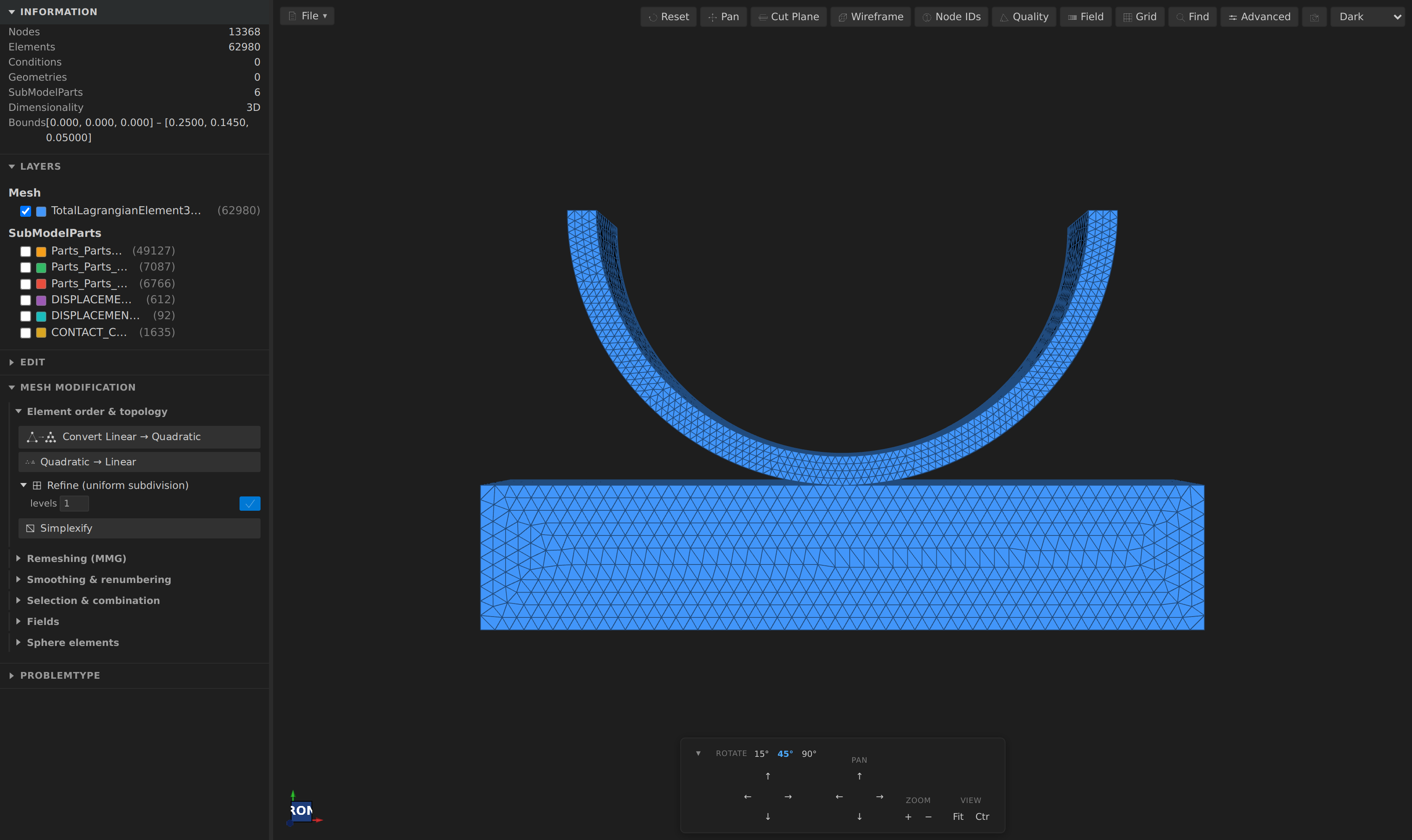
Convert Linear → Quadratic · Quadratic → Linear (the inverse: drops mid-edge nodes) · Refine (uniform subdivision — triangles/quads/tets/hexahedra/wedges split into 4 or 8 children, lines into 2, up to 4 levels, with shared edges/faces deduplicated to a single new node and nodal fields interpolated exactly) · Simplexify (hexahedra/wedges/pyramids/quads → tetrahedra/triangles) · Remesh surface (redistribute) (ACVD: a new triangulation with exactly N vertices, isotropic / curvature-aware / anisotropic; every face inherits block, property, SubModelPart membership and cell fields from the nearest original face, and the message reports the deviation from the original surface) · Generate volume mesh (retetrahedralize) (a tetrahedral mesh of a closed surface or volume on a lattice, with the boundary as Conditions inheriting the surface's parts — and an honest report of its quality caveats) · Optimize tetrahedra (2-3 / 3-2 flips and vertex relocation with fixed nodes: untouched tetrahedra keep their ids, blocks, properties and parts) · Repair surface (fix winding, orient closed components outward, fill bounded holes, split non-manifold vertices, weld — adopted in place; filled faces join the source block and are listed in a Repair_Fill SubModelPart, with no element field values invented) |
| Remeshing (MMG) |
Remesh (MMG) · Level-set split (MMG) — described under Remeshing (MMG) above |
| Smoothing & renumbering |
Smooth (Taubin — shrink-free — Laplacian, or ODT (optimal-Delaunay-triangulation, tetrahedra only, which targets element quality rather than surface fairness and is the one to run before a solve), with boundary pinning, feature-edge preservation and an inversion guard; only coordinates move) · Reorder (RCM bandwidth reduction, or Morton/Hilbert space-filling curves for cache locality — a pure reordering of storage order; every node keeps its own id) · Shrinkwrap (project the nodes onto a triangle surface — a file, a SubModelPart of this mesh, or its own skin — with offset, maximum distance, blend, and move-only / keep-fixed parts; a projection rather than a collision-free fit, so folded cells are counted) · Sobolev deformation (apply a smoothed, optionally pinned displacement field through the mesh's own finite-element operators; a constant displacement is preserved exactly) · Mark connected components (each Element's connected-body index as a field, with isolated fragments flagged) · Renumber (compact ids into a gapless run, each entity kind numbered independently as Kratos does — pair it with Reorder for a full RCM renumbering) · Partition (space-filling-curve domain decomposition into N balanced parts, attached as a real Kratos PARTITION_INDEX field, optionally with one SubModelPart per part) |
| Selection & combination |
Crop (keep only the cells inside a bounding box or on one side of a plane, "all nodes" or "any node") · Merge mesh (append one or several mesh files' nodes and cells in a single operation, offsetting ids per kind, wrapping each source in its own SubModelPart, with an optional weld of coincident nodes run once across every seam) |
| Fields |
Field calculator (a new nodal/elemental/conditional field from a formula over coordinates and existing fields — the same safe expression evaluator as the MMG size = ƒ(h) mode, never eval) · Average field (nodal ↔ elemental averaging) · Manage fields (rename, drop, keep only — lossless, and a global reduction follows a renamed source) · Condition field (clamp, normalize or standardize a field's values, per component or by magnitude, with an explicit NaN policy) · Field gradient (gradient / divergence / curl of a nodal field, Green-Gauss or least-squares) · Surface curvature (mean, Gaussian and principal curvature of a surface mesh as nodal fields — a sphere of radius R reads 1/R and 1/R², a wrong-way winding flips the sign of the mean curvature and says so, and a closed surface reports the Gauss–Bonnet check; usable in remesh size formulas, with a Curvature-adaptive preset) · Field Hessian (the second derivative of a scalar nodal field, as its 9 flattened components — a field that is at most linear has an exactly zero Hessian, which is the guarantee to sanity-check against) · Error estimate (Zienkiewicz-Zhu recovery-based indicator, per cell, optionally marking the worst cells for refinement by threshold, fraction or Dörfler bulk — a field the mesh represents exactly has zero error) · Distance to surface (the signed distance from every node to a surface — an imported file, or a SubModelPart already in this mesh, no file needed — negative inside; feed it straight to Level-set split (MMG) to cut the mesh along that surface) · Compare with another mesh (a field against the same field of another file, by entity id or by spatial point sampling, written as signed / absolute / relative difference fields with uncovered entities left as gaps — never compared as 0) · Transfer fields (mass-preserving transfer of another mesh's fields onto this one — the measure-weighted total is what is conserved; nodal data is smoothed through a cell round trip rather than resampled) |
| Sphere elements |
Set element radius — see Sphere / particle elements |
Smooth / Reorder / Partition / Merge mesh / Field gradient / Field Hessian / Error estimate / Distance to surface / Transfer fields run asynchronously with the same inline progress bar and cancel button as MMG; the rest apply instantly. Every one joins the same undoable operation history and JSON recipe as the operations above, and is reachable from mesh_transform for scripting. The Mesh Editing guide has a worked before/after screenshot for each one.
Editing & operation history — the Edit sidebar section records every applied edit and mesh modification into an undoable history: undo / redo / clear plus a clickable list of operations (click any step to partially revert to it). Edit operations are driven by interactive controls in the sidebar: remove orphan nodes, merge coincident nodes (tolerance), and separate scale, translate, and rotate transforms (values entered inline). Deleting a SubModelPart is done from its ✕ button in the outline tree. Every edit and mesh modification joins the same history, and the applied operations can be saved to / loaded from a JSON recipe and replayed on the mesh (Save operations… / Load operations…). Check "Queue operations for one apply" to combine several operations — from any sidebar form — into one sequence: each still lands as its own undoable step, but it's one click of Apply queued steps instead of N.
Reload from disk — File ▸ Reload from disk (Ctrl+Alt+R) re-reads the file, and so does an external change to it or saving it in a text editor. Applied operations survive a reload: the history is re-applied to the new contents instead of being discarded, an op that no longer applies is kept and marked rather than dropped, and the same holds when you step a VTK time series — except that the expensive remeshing operations are marked skipped instead of re-running on every frame, with a Re-apply button to run them deliberately.
Save / Load problem (zip) — File ▸ Save problem… bundles the whole setup into a single portable zip: the original mesh file, the applied edit operations as a recipe, the problemtype case state (<name>.kratoscase.json) and the generated case files (ProjectParameters.json, the materials JSON, MainKratos.py, <name>_case.mdpa) — whichever exist. File ▸ Load problem… extracts such an archive into a folder of your choice, opens the mesh in the preview, replays the bundled edits automatically and restores the case setup — share a .kratosproblem.zip and the recipient gets the exact same problem. Also available as the Save Problem (zip)… / Load Problem (zip)… palette commands.
Keyboard shortcuts, scoped to the preview tab (they never clobber the global VS Code bindings): Ctrl+O Open, Ctrl+S Save, Ctrl+Shift+S Save As, Ctrl+E Export, Ctrl+Alt+R Reload from disk, Ctrl+Alt+S / Ctrl+Alt+O Save/Load problem, Ctrl+Alt+P Screenshot (⌘ variants on macOS) — plus the in-viewport view snaps 1–6 (±X / ±Y / ±Z) and i (isometric).
Editor integration: mdpa language id with // comments, Begin/End folding, and syntax highlighting. The raw text editor stays the default; open the preview from the editor-title button, the explorer context menu, the Open MDPA Preview command, or the Kratos activity-bar sidebar (see above), which works with nothing open at all.
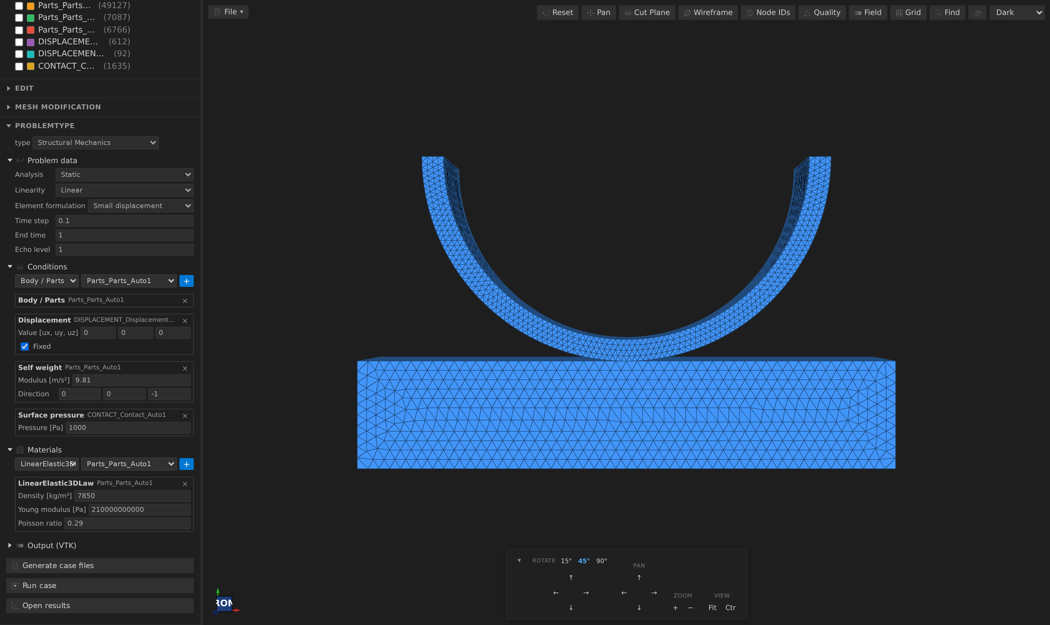
Problemtypes — build & run Kratos cases: the Problemtype sidebar section generates everything a Kratos run needs from the previewed mesh: pick a problemtype (Structural, Fluid, Convection-Diffusion, Potential Flow, Shallow Water built in), fill the solver forms, assign conditions/loads and materials to SubModelParts, and Generate case files writes ProjectParameters.json, the materials JSON and MainKratos.py next to the mesh — which need not be an .mdpa: any previewed mesh format works, and a non-.mdpa mesh is always converted to a <name>_case.mdpa case mesh first, since the solver reads .mdpa. Element/condition block names are adapted to the solver automatically: when the mesh's typology differs from what the chosen physics expects (e.g. SmallDisplacementElement3D4N for structural, generic Element3D4N for fluid), a renamed <name>_case.mdpa copy is generated and the case points at it — the original mesh stays untouched. Output always goes through Kratos' vtk_output_process, so Run case (an integrated terminal with the configured Kratos environment — pip-installed Kratos works with zero setup, and a custom-compiled Kratos is configured with the Select Kratos Installation Folder… command, which auto-detects a source checkout's bin/Release build) produces a vtk_output/ folder the extension previews directly, timeline growing live as steps are written (Open results). The case setup auto-saves to <name>.kratoscase.json and is restored on reopen. Custom problemtypes are plain .js / .py files in .kratos/problemtypes/ (Python runs in bundled Pyodide); faithful Python ports of the five built-ins ship as copyable examples in example/problemtypes/. See the documentation site for the user guide and the authoring API.
Flowgraph node editor (visual case setup): a sixth built-in problemtype, Flowgraph (node editor), embeds the Kratos Flowgraph visual editor directly in the preview. Selecting it splits the view in half and opens Flowgraph in a resizable pane — horizontal (below the mesh) by default, toggleable to vertical (beside it) from the pane header or the kratos.flowgraph.splitOrientation setting. It runs as a bundled local server embedded in an iframe, so the full node editor works unchanged. The bridge is two-way: opening Flowgraph seeds the graph with the current case's ProjectParameters.json, and Flowgraph's Generate writes the resulting ProjectParameters.json back next to the .mdpa, ready for Run case. Flowgraph is AGPL-3.0 — see License.
VTK / mesh file preview
The same viewer opens all common VTK-family and surface-mesh formats, plus 39 more through meshio++:
| Format |
Extensions |
Notes |
| Legacy VTK |
.vtk |
ASCII and binary (big-endian) |
| VTK XML |
.vtu, .vtp, .vti, .vts, .vtr |
ascii, inline base64, appended raw/base64, zlib-compressed |
| VTK multiblock |
.vtm |
referenced blocks merge into one scene; each block becomes a layer; writes back as an index plus one .vtu per top-level part |
| Surface meshes |
.stl (ascii+binary), .obj, .ply (ascii+binary) |
STL vertices are welded; PLY vertex properties become fields |
| Extended (meshio++) |
.msh (Gmsh), .inp (Abaqus), .bdf/.nas/.fem (Nastran), .unv, .mesh (Medit), .vol (Netgen), .su2, .xdmf/.xmf, .off, .dat/.tec (Tecplot), .avs, .f3grid, .pf3, .mfm, .mphtxt (COMSOL), .post/.dato (PERMAS), .ugrid, .wkt, .xml (DOLFIN), .case/.geo (EnSight Gold), .node/.ele (TetGen), .poly (Triangle), .foam (OpenFOAM case: polyMesh plus time-directory fields) |
via @meshioplusplus/wasm 12.0.0. Ambiguous extensions are resolved by content (.msh tries Gmsh then ANSYS/FreeFem; .inp tries Abaqus then ANSYS). Gmsh MSH 4.1 needs ≥ 9.7.0 — earlier builds couldn't read a real-world 4.1 file at all (every such file starts with a $Entities section the reader used to reject on sight), which is also what carries 4.1's physical-group membership, so upgrading also means 4.1 files now get their named regions as SubModelParts. Since 11.5.0 a .msh export also declares $PhysicalNames (untagged groups get freshly allocated tags) instead of dropping them. Export also offers write-only SVG/TikZ figures. OpenFOAM export (meshio++ ≥ 9.20.0) is the one format that writes a directory: picking .foam leaves a 0-byte marker there and puts the mesh in constant/polyMesh/ beside it, with patch names recovered from the model's SubModelParts afterwards (a patch-less mesh still gets the single synthesized defaultFaces) |
| GiD postprocess (meshio++) |
.post.msh + .post.res (ascii pair), .post.bin (deflated), .post.h5 (HDF5) |
Kratos's reference pre/post-processor, readable and writable since meshio++ ≥ 10.19.0 / 10.18.0. Multi-step: the steps live in the .post.res headers and drive the timeline bar, like Exodus. These are compound extensions — case.post.msh resolves to GiD, not to .msh/Gmsh, and a bare .post is PERMAS as before. Opening either half of the ascii pair finds the other. Export offers the ascii flavour, which writes both files |
| HDF5 / netCDF containers (meshio++) |
.cgns, .h5m (MOAB), .hmf, .med (Salome), .e/.exo/.ex2 (Exodus II) |
needs a meshio++ ≥ 8.0.0 build (Exodus ≥ 8.6.0, for real SEACAS/Cubit/Sierra files — earlier builds threw on the qa_records every such file carries). MED's named groups (*FAS/*GRO families) become SubModelParts too, since meshio++ ≥ 9.6.0, and a real Salome/Code_Aster file that the strict reader refuses is retried leniently (meshio++ ≥ 9.9.0) instead of failing to open. .med can now be written (meshio++ ≥ 9.9.0, which fixed the vector-field shape bug that made every earlier writer fail on the common case): fields survive scalar and vector alike, and SubModelParts arrive as MED families. CGNS now carries point and cell data (meshio++ ≥ 9.9.0 — earlier it silently dropped every field), and has been a genuine CGNS/SIDS-compliant writer since ≥ 9.8.0 (before that it wrote only the first tetra block it found, so any other mesh — every surface mesh included — produced a file nothing could read). Exodus can be written (meshio++ ≥ 9.3.0) but lossily, so pick it knowingly: element blocks, point_data and per-element data all survive (vectors included since ≥ 9.9.0), and block names now round-trip as SubModelParts, but a genuine SubModelPart does not — the writer emits no node sets or side sets — a time series is flattened to one step, and the output is NetCDF-4/HDF5 rather than classic netCDF-3. Export to .mdpa/.vtu/.med if the grouping matters. Exodus carries its own in-file time series — see Timeline animation — and its element blocks/node sets/side sets become SubModelParts like every other format's named groups. .xdmf written from the extension now emits a companion <stem>.h5 beside the XML — both files are needed to re-open it |
Named groups become SubModelParts. Gmsh physical groups, Abaqus *NSET/*ELSET/*SURFACE, and every other named group meshio++ recognizes arrive as SubModelParts in the outline tree, with the usual frame / export / rename / delete / organize actions. A surface group (a set of cell facets rather than whole cells) is materialized into real boundary-facet Conditions, so it is a visible layer — and exporting to .mdpa yields genuine Kratos Conditions.
Filename-based playback supports VTK, STL, OBJ, PLY and the extended meshio++ formats that do not already have an in-file timeline. Open a file named <prefix>_<rank>_<step>.<ext> (for example Main_0_2.ply) to discover its sibling steps. Groups stay separate by extension; the selected frame uses the usual reader and companion files. Existing root-file groups survive subpart merging.
Point/cell data arrays from any format appear in the Field panel; mesh quality, find-by-ID, and screenshots work everywhere.
Submodelpart tree
The sidebar shows the same layer tree as the MDPA preview. The root model-part file provides the full mesh; each submodelpart file (e.g. FixedEdgeNodes, MovingNodes) appears as a hidden-by-default overlay layer that you can toggle independently. Point-cloud submodelparts (node-only files) are rendered as vertex cells.
Timeline animation
When multiple time steps are found in the directory, a timeline bar appears at the bottom of the viewport:
◀ ▶ ▶▶ ══════●══════════ Step 4 (2/3) 2 fps
- ◀ / ▶▶ step backward / forward one frame
- ▶ / ⏸ play / pause (at the configured fps rate)
- Scrubber — drag to jump to any step instantly
- fps input — controls playback speed (1–30 fps)
Camera position, layer visibility, active field variable, and colormap are all preserved when switching frames. A single file with no timestep siblings opens as a static preview with no timeline bar. Filename-based grouping covers VTK, STL/OBJ/PLY and meshio formats without an in-file timeline.
Exodus, GiD postprocess, MED, CGNS, Tecplot and XDMF carry their own steps, while OpenFOAM lists numeric time directories. These drive the same timeline bar without a filename grammar, and newly appended steps extend the timeline live. MED, CGNS and Tecplot enumerate their steps since meshio++ 11.3.0 (native metadata readers); Gmsh selects steps but cannot enumerate untagged sections, so it stays on filename grouping.
The Advanced toolbar button holds operations that are useful but not everyday, so the toolbar does not grow a button per niche feature.
Mesh size
Opens the Mesh Size panel — per-node and per-element size statistics, a box-and-whisker plot, and smallest/largest highlighting. See Mesh Size above for the full details.
Face normals
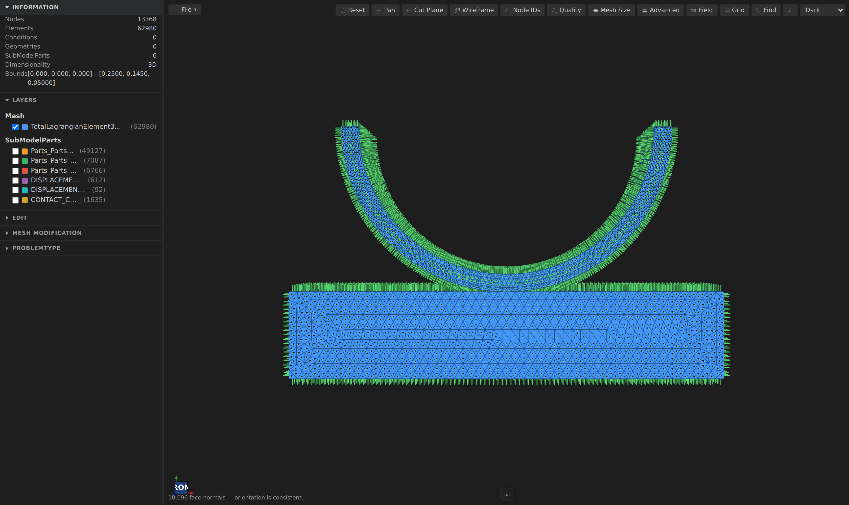
Draws an arrow on every surface face and every boundary face of a volume mesh. This is the standard way to find an inverted element: the winding of a cell decides both the arrow direction and the sign of its Jacobian, so a flipped cell points against its neighbours — obvious on screen, invisible in the numbers, and a hard error for the solver.
Hole rims are outlined in orange and non-manifold edges in violet, so a defect has a place and not just a count. Faces wound against a neighbour are also counted and highlighted in red, and the status line reports whether the orientation is consistent. Note this is a relative test: a mesh that is uniformly inside-out is self-consistent and reports none, so the arrows themselves remain the check for global orientation.
Run manager
Running a case used to be fire-and-forget: the extension launched a terminal and said "running" forever, whatever actually happened. Now every run is tracked in a Kratos Runs view in the Explorer, with its status, elapsed time, the latest step written to vtk_output/, and — when it ends — a real exit code.
The solver runs as a child process with its output in an Output channel, which is what makes the exit code, the live progress and a working Stop possible; it also fixes a launch failure being reported properly, so a wrong kratos.pythonPath now names itself instead of scrolling past in a terminal. Set kratos.run.launchMode to terminal if you need an interactive shell instead — such a run is still listed, but marked detached, because a terminal cannot report when the solver exits and the extension will not claim otherwise.
Stopping interrupts the solver so it can close the file it is writing; anything already in vtk_output/ is kept. Because the last step of an interrupted run may be half-written, Open results for a run that did not finish cleanly opens the last complete step.
Runs outlive the preview that started them. If the window is closed or reloaded they are stopped by default (kratos.run.stopOnWindowClose), and whatever is found afterwards is reported honestly: a run whose process is gone reads orphaned, and one whose process may still be alive reads detached — never running, because process ids get reused and the extension will not claim a liveness it cannot verify. Agents drive the same runs through the case_run, case_status and case_stop MCP tools, which meet the editor on the same sidecar file — so a run started on either side is visible from both.
Record a video
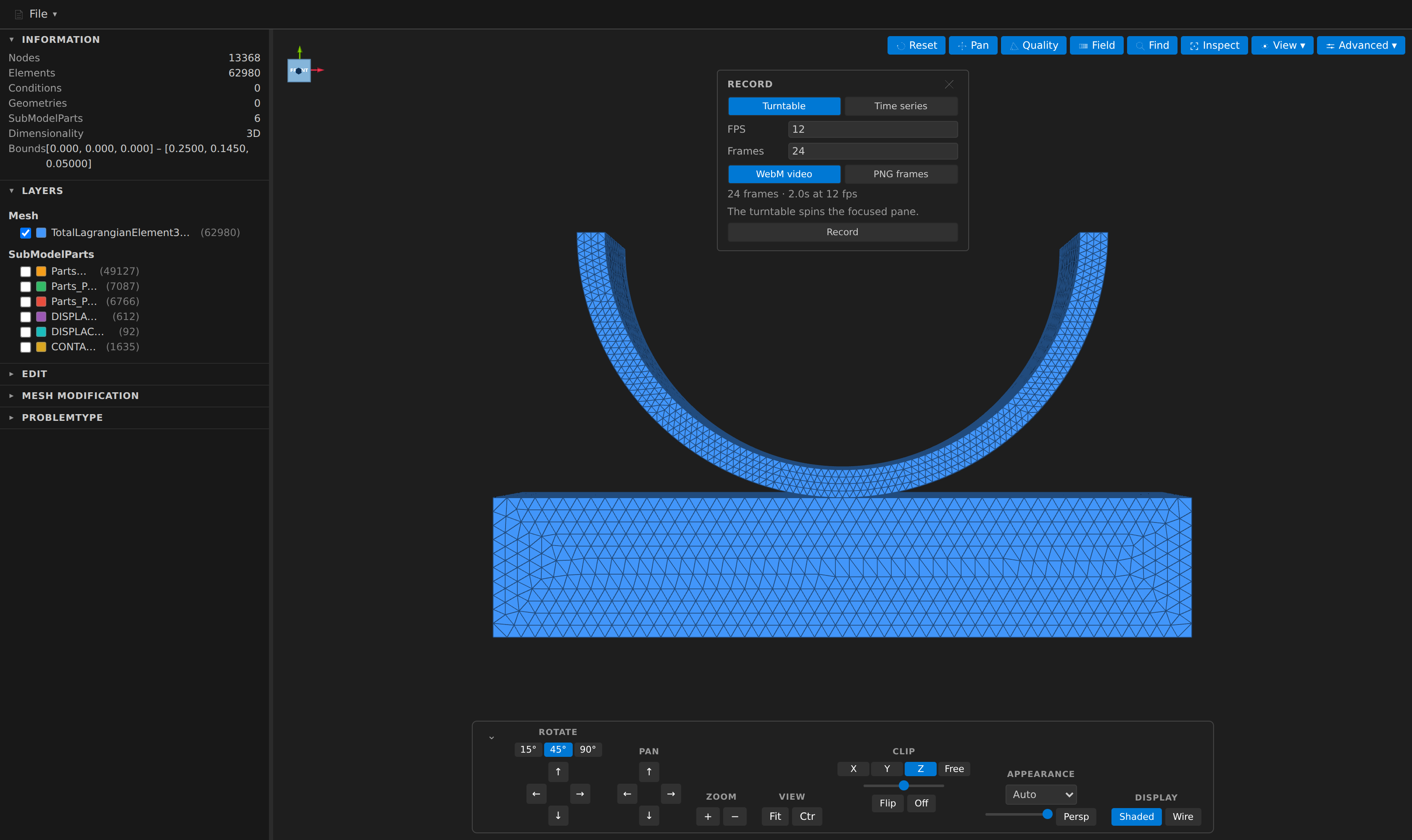
View ▾ ▸ Record… turns the viewport into an animation. Two sources: a turntable that spins the camera through one full revolution (available for any mesh, including .mdpa files with no time dimension), and a time series playthrough that steps through every frame of a mesh series.
The result is a WebM video, or a numbered PNG sequence if you would rather encode it yourself — the extension prints the exact ffmpeg -i <stem>_%04d.png out.mp4 line when it saves them. mp4 is not offered directly because the browser engine VS Code is built on cannot reliably encode H.264; the PNG route is the honest answer rather than a format that sometimes fails.
Each frame is captured only once the frame it depends on is genuinely on screen, so a recording of a time series is a faithful playthrough rather than whatever happened to be drawn when a timer fired — worth knowing because every step of a series is a full re-read from disk, so a long recording takes real time. The progress bar counts frames, and Cancel keeps whatever was captured.
In a split view the recording includes every pane, with the pane separators drawn in so it matches what is on screen. A turntable spins the focused pane.
Split view
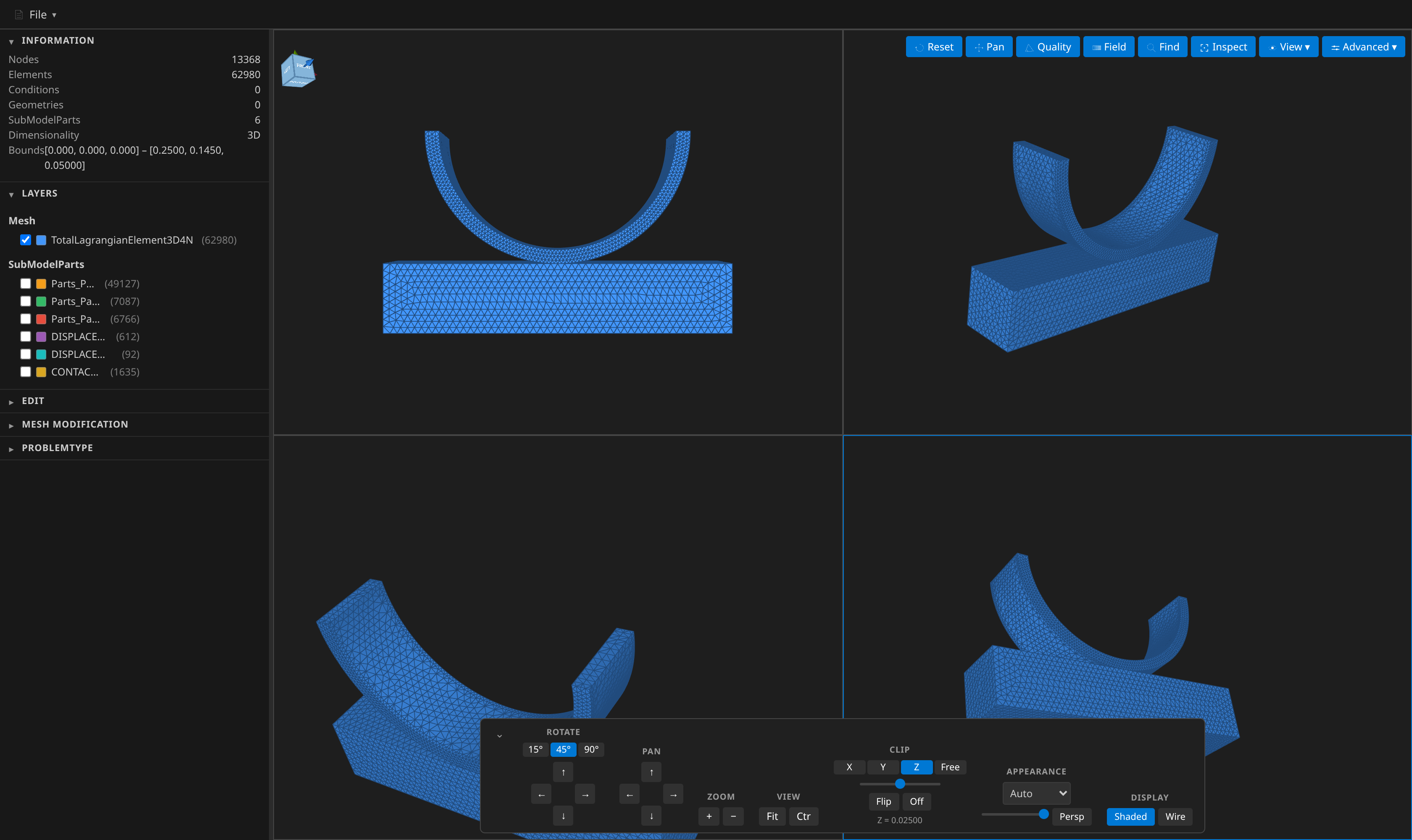
View ▾ ▸ Layout splits the viewport into 1, 2 or 4 panes. Each pane has its own camera over the same mesh, so you can look at the front and the top at the same time, or keep an overview beside a zoomed-in detail, without reloading anything.
Orbit, pan and zoom apply to the pane under the pointer. The pane you last pressed in is outlined, and that is the one Reset, Frame, the navigation dock and the keyboard view shortcuts act on — the orientation cube also turns to match it.
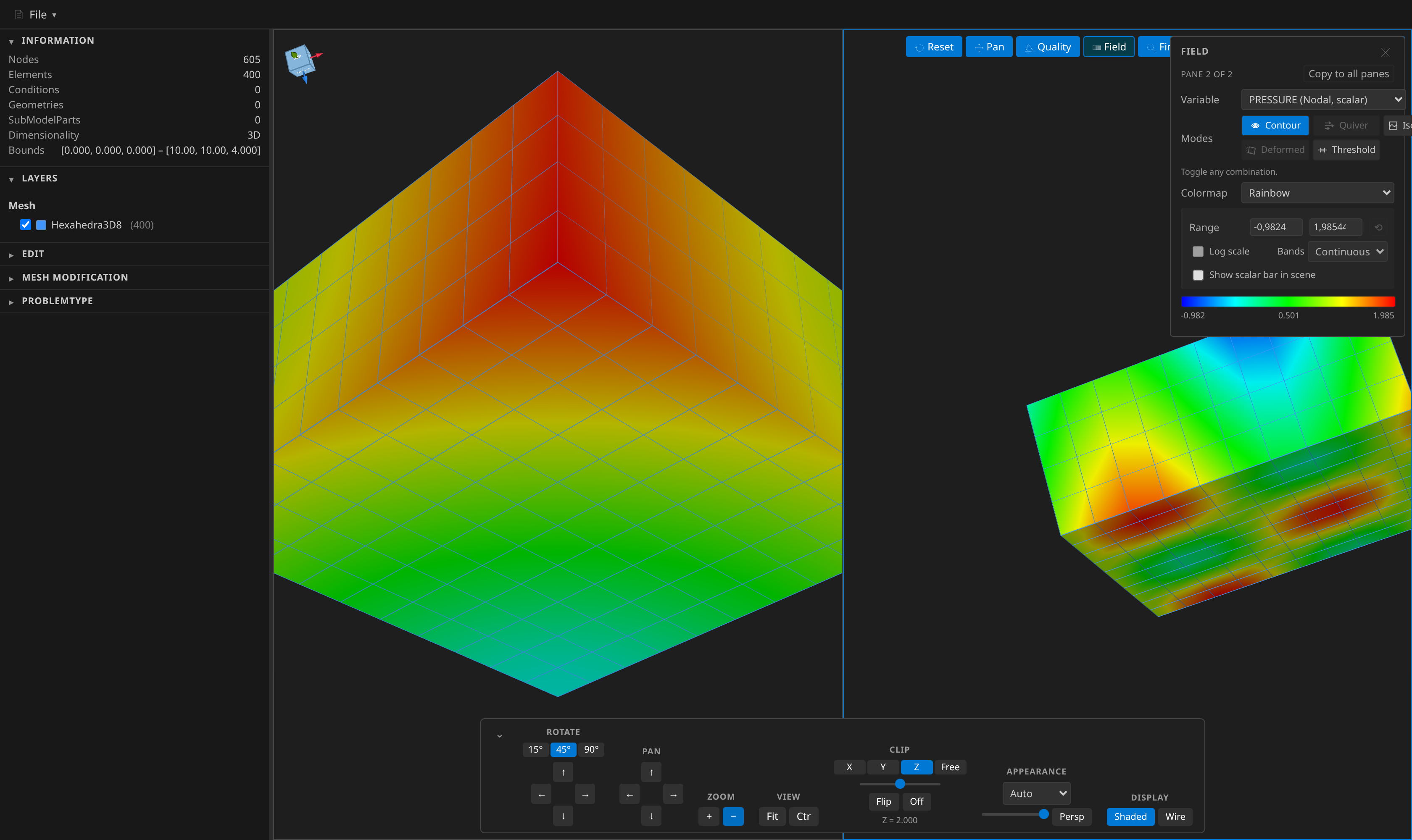
The Field panel and the Clip controls also act on the focused pane, so each pane can show a different variable, colormap, component, range, isosurface, threshold or deformation, and its own clip plane — the panel names the pane it is editing and offers Copy to all panes when you want them to agree. Click into a pane to point the panel at it.
Everything else stays shared: the same layers, visibility, colours, opacity and display mode appear in every pane, so a split is a second viewpoint rather than a second document. A screenshot captures the whole grid; in a split, switch on Show scalar bar in scene so each pane's legend is part of the picture.
Node IDs are shown in the single-pane layout only: they are drawn as HTML labels projected through one camera, so in a split they would land over the wrong panes.
Plot over time
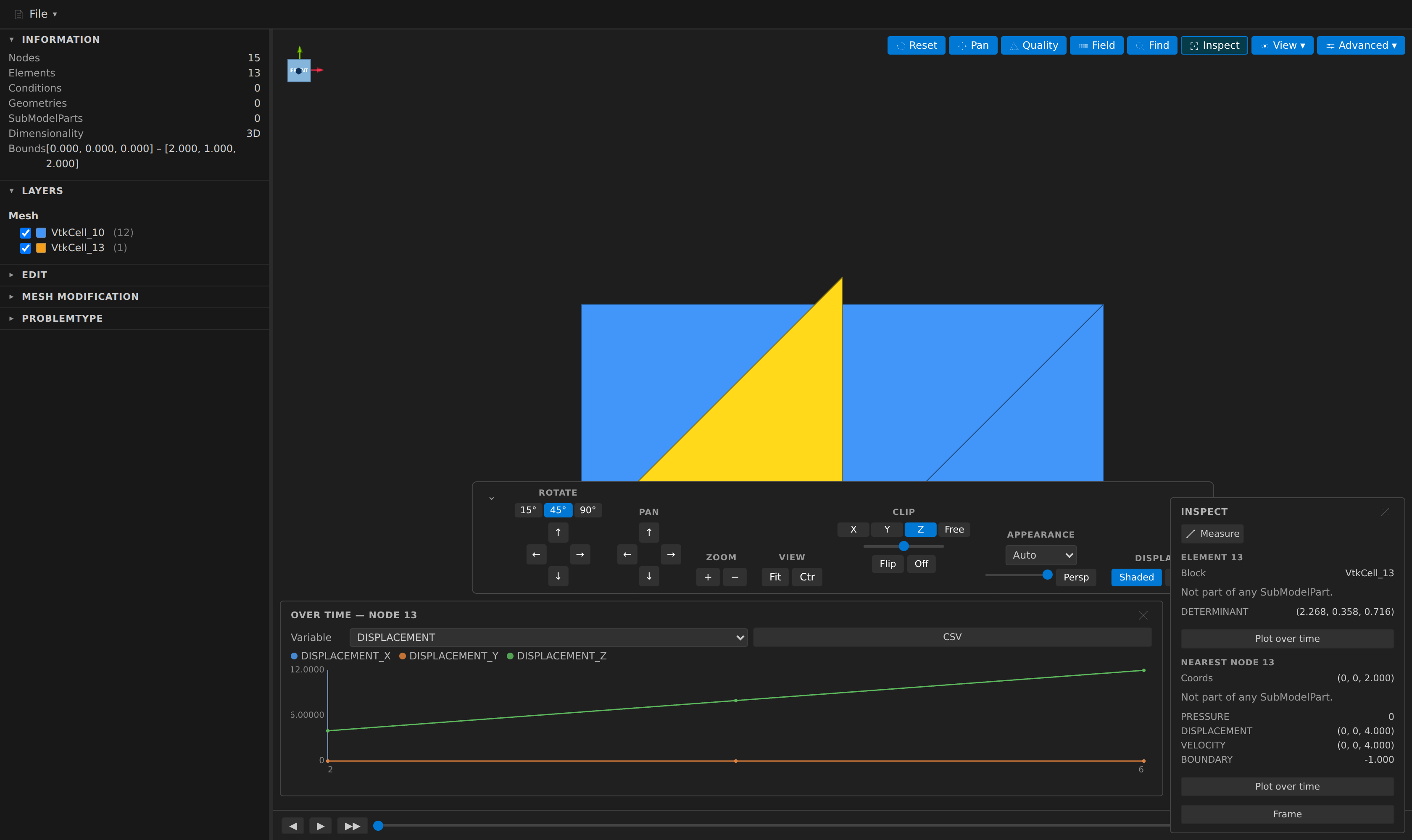
Reading one number at one step is what Inspect does. This answers the other half: what that number did across the whole run. Pick a node or element, choose a variable, and the extension reads every step of the time series and charts it.
The scan runs in the extension host, not in the preview — the viewer only ever holds one frame, so charting from it would mean stepping the whole timeline and watching the viewport flicker through every frame to read one value. Progress is shown per step and the scan can be cancelled; a partial series is still plotted.
What it will not do is quietly make the data look tidier than it is. A step where the variable is not written, or where the entity does not exist, leaves a break in the line rather than a segment drawn through it, and the panel says how many steps were missing and which of the two reasons applied. If the mesh changes size partway through the series, it says that too — the id still resolves, but it may no longer be the same entity. Edit operations from the sidebar are not replayed per step (that would cost as much as scrubbing the timeline by hand), so if any are applied the panel tells you the values are the ones on disk.
Clicking a point jumps the 3D view to that step. CSV saves the series. Also available headlessly as the mesh_field_series MCP tool.
Data table
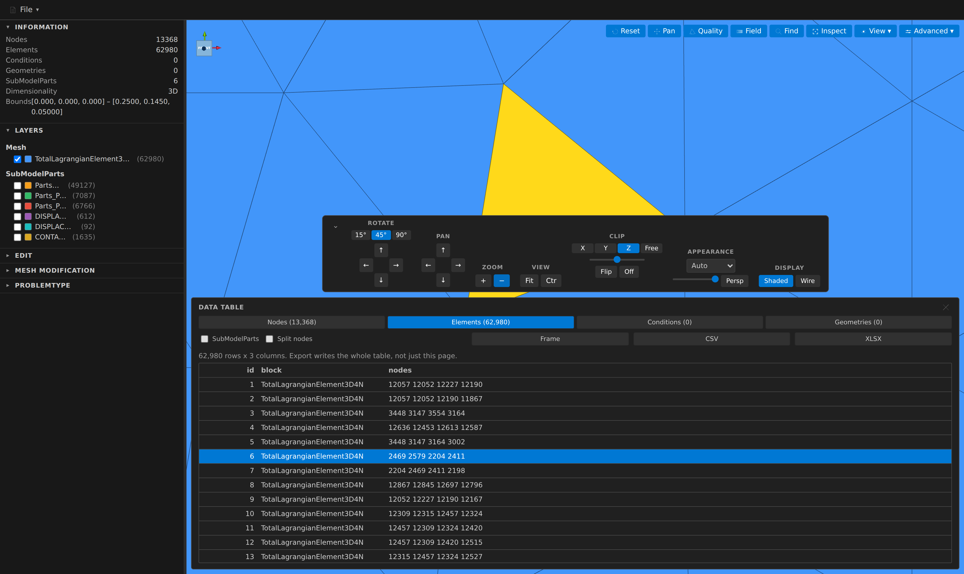
Every node, element, condition or geometry as a row of plain values — the id, the coordinates (nodes) or the block and connectivity (entities), optionally the SubModelParts it belongs to, and every field defined at it. A vector field splits into NAME_X/NAME_Y/NAME_Z columns (a wider one, such as a Hessian, into NAME_0…NAME_n), and a field that does not cover a row leaves the cell blank rather than showing a zero the mesh does not carry.
Clicking a row highlights and frames that entity in the 3D view, so a number in the table can be found in the mesh without leaving the panel. The table paginates at 100 000 rows and renders only the visible window, so it opens on a multi-million-entity mesh as quickly as on a small one.
CSV and XLSX export always write the whole table, not the visible page. CSV is streamed, so it has no size limit beyond your disk; XLSX is capped by Excel's own worksheet limit (1 048 576 rows) and tells you when it had to leave rows out. Coordinates export at their true float32 precision rather than the 0.10000000149011612-style expansion a naive conversion produces. Also reachable from the Command Palette (Kratos Mesh: Export Data Table) and from the mesh_export_table MCP tool.
Export skin
Extracts the boundary of the mesh's volume cells (plus any pre-existing surface cells) as a standalone surface mesh and writes it to a file of your choice, via the same format picker as File ▸ Export. Unlike meshio++'s own surface/skin extractors, this is a native boundary-face walk — a face seen by exactly one cell is boundary — so SubModelParts survive the extraction, narrowed to node membership (element/condition membership cannot follow, since the skin's faces get fresh entity ids with no correspondence to the source mesh). Also reachable from the mesh_extract_skin MCP tool.
Simplify surface and Level of detail
Advanced ▸ Simplify surface… writes a decimated copy of a triangle surface (quadric-error edge collapse): boundary and crease vertices are pinned, surviving faces keep their entity ids, property ids and cell-field values, and the report gives the reduction and the largest collapse error as a share of the bounding-box diagonal. View ▸ Level of detail draws a decimated surface in place of the full layers to keep a huge mesh navigable — the mesh is untouched and picking is off while it shows. mesh_derive (kind: "decimate") is the headless route.
Sample to grid
Advanced ▸ Sample to grid… (or Kratos Mesh: Sample to Grid) samples the surface — or the boundary skin of a solid — onto a regular lattice and writes it as a new file: a voxel occupancy (cells whose centre is inside the surface, with a VOXEL_OCCUPANCY 0/1 field) or a signed-distance volume (the distance to the surface at every lattice point, negative inside, as SDF_DISTANCE). It asks for the cell size, shows the cell count and memory it implies before anything is allocated, confirms above five million cells and refuses beyond twenty million. A complete lattice can be written as .vti — the only container that keeps the sdf:* header (origin, spacing, dimensions) — while a partial voxelization or an octree goes to .vtu or another cell format. This complements the Signed distance operation, which samples only the open mesh's own nodes. The same builders are the grid, voxelize and sdfVolume kinds of mesh_derive.
Export partitions and Split mesh
Advanced ▸ Export partitions… writes the mesh as N per-part files plus a manifest, with optional ghost layers: every cell is owned by exactly one part, each part is rebuilt natively from the source cell ids so ids, kinds, Properties, SubModelParts and fields all survive, ghosts are flagged (PARTITION_GHOST, a Ghost SubModelPart, PARTITION_INDEX = the owner), and the manifest lists interface nodes and imbalance. Split mesh… writes one file per connected body, element type or field value. The WebAssembly build has no KaHIP, so the cut is a space-filling curve. Both are the mesh_split MCP tool.
Sphere / particle elements
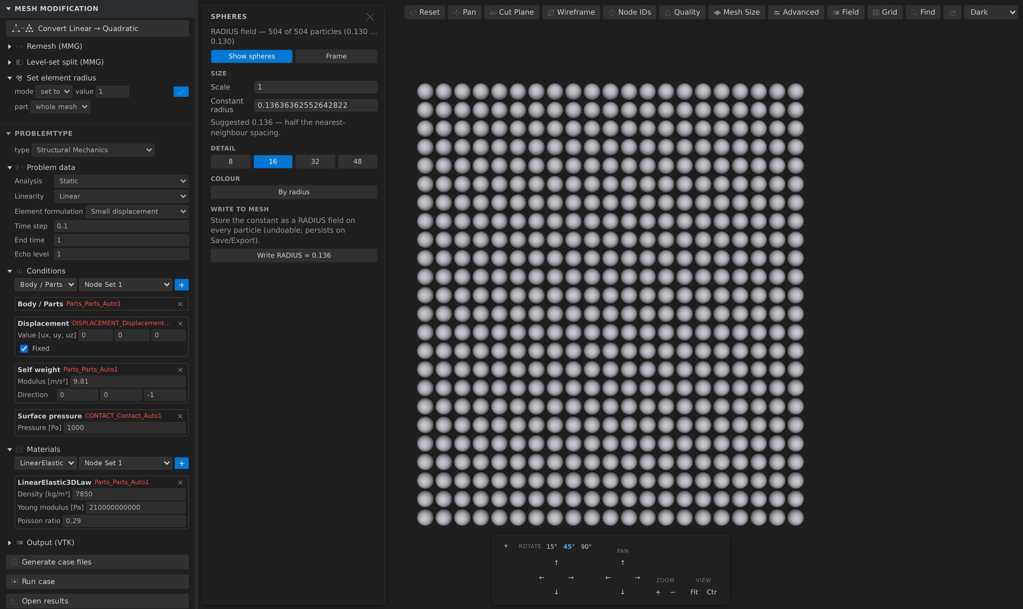
Peridynamics and DEM meshes are made of one-node elements — Exodus writes them as SPHERE, Kratos DEM as spherical particles. They have no extent, so by default they draw as fixed-size screen points, which tells you nothing about how big the particles actually are.
The Spheres toolbar button renders them as real spheres instead, scaled in model space so they behave like geometry under zoom:
- RADIUS field — when the mesh carries one (an Exodus per-element
RADIUS attribute arrives as an Elemental field of that name), every particle is drawn at its own radius, and the rendering turns on automatically.
- Constant radius — most particle files carry no radius at all. The panel suggests one (half the median nearest-neighbour spacing, so touching particles read as touching) and you can override it.
- Scale, detail (sphere tessellation) and optional colour by radius.
- Write to mesh turns the constant into a real
RADIUS field. It is a normal, undoable mesh operation, so it saves, exports and appears in a saved recipe — also reachable from the Set element radius form in the Mesh Modification sidebar (which can also scale existing radii, and can target a single SubModelPart), and from the mesh_transform MCP tool.
Exporting such a mesh to .exo writes the radius back as an Exodus element attribute; exporting to .mdpa writes a Begin ElementalData RADIUS block.
Beam / line elements
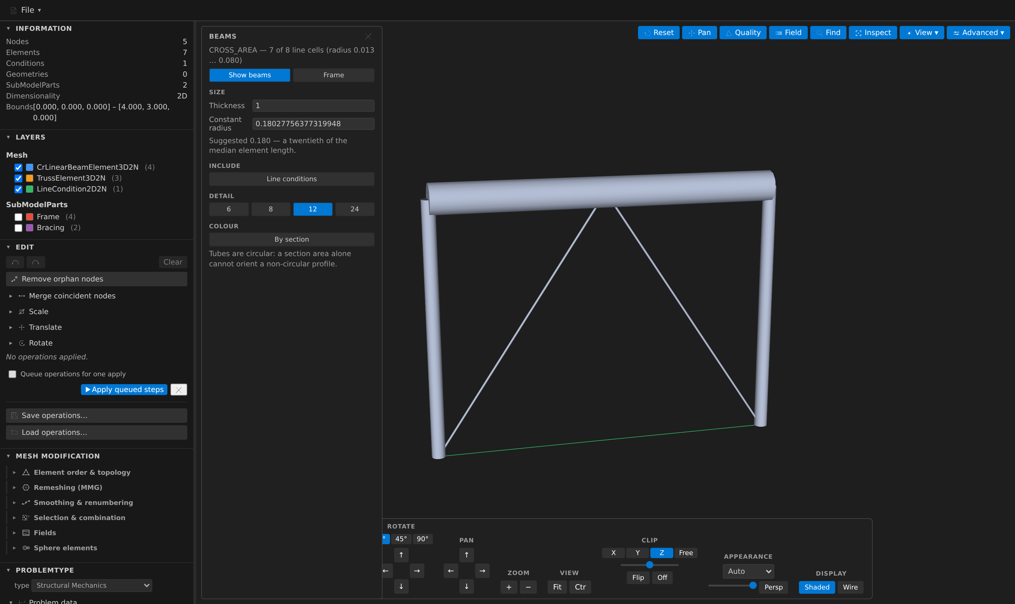
A frame or a truss is made of line elements with a cross-section. They have no extent either, so by default they draw as fixed-width screen polylines — a 6 mm tie rod and a 600 mm girder look identical at every zoom.
Advanced ▸ Beams… draws them as real tubes, scaled in model space:
CROSS_AREA from the Properties block — where Kratos actually keeps a member's section. The drawn radius is the circular-equivalent sqrt(A / π), resolved per cell (repeated Begin Elements blocks merge into one layer, so a single layer routinely holds members on several properties). An ElementalData CROSS_AREA field is used when Properties carry none.- Constant radius — a twentieth of the median element length, for a mesh that declares no section.
- Thickness multiplies the radius only, never the length, so a member never detaches from its end nodes. Plus tessellation and optional colour by section.
A line cell is also the shape a 2D boundary takes, so the rendering only turns itself on when the mesh gives it a reason to: the section must be a real CROSS_AREA, and only Elements count towards enabling it — a LineCondition2D2N skin that happens to share a structural part's property id never flips it on. Draw such conditions deliberately with Line conditions.
The section is read, not written: it belongs in Properties, which a Save emits from the model. mesh_info reports a properties section with the parsed values, and a beams section describing the line cells. See example/MDPA/portal_frame.mdpa.
Known limitations
- MPI rank > 0 files are not merged in this release (rank-0 files are loaded).
- Submodelpart merging uses coordinate matching (
toFixed(6)); if the root and subpart files were written at different float precision the merge may miss nodes (a diagnostic is emitted in the sidebar stats).
MCP server
The extension ships a standalone MCP server (dist/mcpServer.js) that exposes its mesh and simulation-setup engine to any MCP client (Claude Code, Claude Desktop, …) — no VS Code needed. Build it once with npm run compile, then register it, e.g. with Claude Code:
claude mcp add kratos-mdpa -- node /abs/path/to/VSCode-MDPA-Preview/dist/mcpServer.js
or in a generic client config:
{ "mcpServers": { "kratos-mdpa": { "command": "node", "args": ["/abs/path/to/dist/mcpServer.js"] } } }
| Tool |
What it does |
mesh_info |
Parse any supported mesh (.mdpa, VTK family, .stl/.obj/.ply, and the extended meshio++ formats) and summarize nodes, blocks, SubModelParts, fields, diagnostics. Named groups from formats that carry them (gmsh physical groups, Abaqus sets, Exodus blocks/node sets/side sets) appear as SubModelParts. inputFormat forces a reader no extension defaults to (ansys, freefem, ansysinp). timeStep selects a step of a multi-step mesh (Exodus, MED since meshio++ 9.9.0, GiD postprocess, CGNS/Tecplot since 11.3.0, XDMF, OpenFOAM time directories); the response then includes timeStep/timeValues (Exodus, GiD, MED, CGNS, Tecplot, XDMF and OpenFOAM list theirs). metadataOnly skips parsing and reports the file header (counts, block shapes, data-array names, regions, bbox) for the formats whose reader stays header-only (.xdmf/.xmf, .msh, .med, .cgns, .dat/.tec, the GiD .post.* set) — anything else is refused rather than served at header price. An OpenFOAM case is opened through its .foam marker, like any other path. summary is the universal counterpart: it reports the file shape for every supported format, including .mdpa and the natively-parsed VTK/STL/OBJ/PLY, and never refuses for ineligibility — it reports cost instead (header a bounded read, scan a whole-file stream that builds nothing, buffered/read the meshio++ paths that hold or parse the file), with bytesRead saying what it actually took and unknown naming what the format cannot report so a blank is not read as a zero. A mesh with one-node (sphere/particle) elements also reports a spheres section — how many, whether they carry a RADIUS, and a suggested radius if not. An .mdpa that declares Begin Properties also reports a properties section with the parsed values, one that declares Begin Constraints a constraints section (per block: name, variables, row count and id range, plus undefinedIds — constraint ids a SubModelPart lists that no block defines), and a mesh with line cells a beams section (how many carry a CROSS_AREA, and how many of those are Elements rather than boundary conditions) |
mesh_quality |
Geometric quality metrics (edge ratio, angles, gradation) with Kratos thresholds and worst-element ids, plus a watertight section: how many boundary edges (holes), non-manifold edges, inconsistently wound face pairs and zero-area faces — the counts rather than a bare flag, since three boundary edges is a pinhole and three thousand is a surface that was never closed |
mesh_size |
Nodal size (NODAL_H, a port of Kratos FindNodalHProcess) + element size (mean edge length), with box-whisker statistics and the IQR-outlier smallest/largest element ids |
mesh_field_integrate |
Cell-measure-weighted total and mean of the cell fields — a density field's total mass, a flux field's total power, an occupied volume — for the whole mesh and per named region, which here means one row per entity block and one per SubModelPart. Regions overlap rather than partition, so their totals need not sum to the domain total |
mesh_curvature |
Discrete mean / Gaussian / principal curvature statistics of a surface mesh, the Gauss–Bonnet check (angle-defect sum vs 2πχ), boundary / isolated / degenerate node counts and orientation warnings — read-only; mesh_transform's curvature op writes the fields |
mesh_compare |
Compare two meshes and their fields by entity id: a verdict (identical / equal within tolerance / different), moved nodes with the worst id, entities only in one mesh or with changed connectivity or type per kind, block-name and SubModelPart-membership differences, and per-field max / mean / RMS / relative error with coverage gaps counted (never compared as 0). With variable it also compares one field — by id, or by spatial point sampling of the other mesh's nodal field — and with outputPath writes the difference mesh (<name>_DIFF, _ABS, _REL) |
mesh_derive |
Write a new mesh derived from the opened one (nothing is written back to the input): a slice through a plane, the isosurface of a nodal field, a threshold region where a field lies in an absolute or normalized window, a decimated copy of a triangle surface, or a regular sampling of it — grid (a lattice from nothing, no input mesh needed), voxelize (occupancy) and sdfVolume (signed distance, dense or octree), sized by cellSize or resolution with a memory estimate and a 20-million-cell refusal before anything runs; a complete lattice can be written as .vti. Slices and isosurfaces carry the interpolated fields and tag every cell with the cell it was cut from (SOURCE_ENTITY_ID / SOURCE_ENTITY_KIND); a threshold region keeps original ids, groups, fields, Properties and the conditions still on it, or returns its boundary surface. Normalized windows need an explicit fixed reference range — rescaling per frame is opt-in |
mesh_probe |
Sample a nodal field along a polyline — distance-versus-value rows with a gap (null) wherever the path leaves the mesh or crosses a region the field was never written, never a fabricated 0 — optionally across every step of a time series, with CSV output |
mesh_split |
Split one mesh into several files that keep the source's ids, kinds, Properties, SubModelParts and fields: partition writes N per-part meshes with optional ghost layers (every cell owned by exactly one part, ghosts flagged, weights by an elemental field, interface nodes and imbalance in the manifest — space-filling curve only, the WebAssembly build has no KaHIP), or component / type / field split into connected bodies, element types or field values |
mesh_transform |
Apply a sequence of mesh operations (scale/translate/rotate, merge nodes, remove orphans, linear→quadratic, delete/rename SubModelPart, reorganize the SubModelPart tree (create / move / merge / add / remove entities), write mesh-size fields, set/scale the sphere-element RADIUS, MMG remesh & level-set split, smooth, reorder, partition, refine, simplexify, linear→linear-only (quadratic→linear), crop, field calculator + nodal/elemental averaging, field gradient/divergence/curl, field Hessian, Zienkiewicz-Zhu error estimate, signed distance to a surface (an imported file, or a SubModelPart already in the mesh), mass-preserving field transfer from another mesh, merge another mesh file) inline or from a saved Edit-sidebar recipe |
mesh_convert |
Convert between formats — ours (.mdpa, .vtk, .vtu, .vtp, .stl, .obj, .ply) plus ~35 written by meshio++ (.msh, .inp, .bdf, .unv, .mesh, .vol, .su2, .xdmf, .off, .poly (Triangle), the HDF5 containers .cgns/.h5m/.hmf/.med, plus the field-only .dex/.ip/.mff and write-only .svg/.tikz figures, …); plus .e/.exo/.ex2 (Exodus, lossy — see the format table). inputFormat/outputFormat override the extension defaults; timeStep selects a step of a multi-step input (Exodus, MED, GiD postprocess, CGNS/Tecplot, XDMF, OpenFOAM time directories). Writing .xdmf also emits a companion <stem>.h5 |
mesh_extract_submodelpart |
Slice one SubModelPart (+ subtree) into a standalone file |
mesh_extract_skin |
Extract the boundary skin of a mesh's volume cells (+ any pre-existing surface cells) as a standalone surface mesh — a native boundary-face walk, so SubModelParts survive (narrowed to node membership) |
mesh_field_series |
One entity's value for one variable across every step of a time series — the headless mirror of the viewer's Plot over time, and the only tool that reads a value across steps. Steps are discovered from a single path exactly as the preview does (a sibling <prefix>_<rank>_<step> series (VTK, STL/OBJ/PLY and meshio formats without an in-file timeline), an in-file series such as Exodus/GiD/XDMF/OpenFOAM, or a lone file), and source reports which was found. A gap is null, never 0, with missingField and missingId counted apart; topologyChangedAt warns that the mesh changed size mid-series. Writes a .csv when outputPath is given |
mesh_export_table |
Tabulate every node/element/condition/geometry as rows of plain values — id, coordinates or block+connectivity, optional SubModelPart membership, and every field defined there. The only tool that reports field values (mesh_info reports field metadata; mesh_find_entity answers for one id). With outputPath it writes the whole table as .csv/.xlsx; without one it returns limit rows from offset as JSON (default 100, max 10 000). submodelpart restricts rows to one part and its subtree |
mesh_pack_series |
Packs a solver run's per-step mesh files into ONE transient XDMF time series. path is the vtk_output directory or any one step file; steps are found the same way the preview finds them (<prefix>_<rank>_<step>), and the step label becomes the time, so the axis carries the Kratos step numbers rather than 0..N-1. Not mesh_convert with outputFormat: xdmf — that writes ONE mesh, this writes every step. Only .xdmf/.xmf are accepted (the one format that carries a mesh time series) and the sibling .h5 is part of the output, not an extra. Refuses a lone file, a format that already carries its own steps, and a series whose mesh changes between steps (an XDMF series has one grid for all steps). Streams one step at a time, and the result re-opens in the preview as a timeline. |
mesh_find_entity |
Locate a node/element/condition/geometry by id (coordinates, connectivity, owning SubModelParts) |
mesh_capabilities |
meshio++ capability inventory: the installed WASM build's readers/writers, per-reader options-awareness, backend and cgnslib — next to the extension's routing (read candidates, write targets, in-file vs filename timelines, header-only metadata set, unrouted keys with reasons) and a fidelity section (the carry/adopt adapter's carrier keys, SubModelPart region prefix, and which model slots it retains). Takes no arguments |
problemtype_list / problemtype_describe |
Enumerate built-in + workspace problemtypes; get the full form/condition/material spec plus a default case skeleton |
case_run |
Start a Kratos solve (generating the case files first unless told not to). The solver is always spawned detached, with its output appended to <stem>.kratosrun.log, so it outlives the MCP server — which cannot own a run, since its stdout is the protocol channel. waitSeconds (default 10, 0 = don't wait) blocks for the exit; expiry is not an error but a handoff, returning running with the pid and log path, since the only applicable timeout belongs to the client and the server cannot observe it. Refuses to start over a run that may still be active unless forced. python / installPath / extraEnv are arguments, defaulting to a pip-installed Kratos |
case_stop |
Stop the latest run by the pid in its sidecar, escalating SIGINT → SIGTERM → SIGKILL (Windows: immediate terminate — signals are not real there) and reporting which rung worked — SIGINT is what lets python close its last result file rather than truncate it. Records the stop before signalling so it reads cancelled, not failed. A run that already ended is never signalled, since pids get reused |
case_status |
The latest Kratos run for a mesh: status, exit code, command, pid and a vtk_output/ summary. Reads the <stem>.kratosrun.json sidecar, so either side can see what the other started — and reconciles it against the OS rather than repeating it, so a stale record whose process is gone reads orphaned and one whose pid is alive reads detached, never running |
case_validate / case_write_state |
Check a case setup against mesh + problemtype; write <stem>.kratoscase.json (picked up by the sidebar) |
case_generate |
Write ProjectParameters.json, the materials JSON and MainKratos.py next to the mesh — same output as the sidebar's Generate button, including solver mesh-name adaptation (a non-.mdpa mesh is always converted to <stem>_case.mdpa first) |
problem_pack / problem_unpack |
Bundle the whole problem (mesh + edit recipe + case state + generated case files) into one zip, or extract such an archive — the same format as the File menu's Save problem… / Load problem… |
MMG operations run in-process and block the server while they run; progress is streamed as MCP log messages.
Develop
npm install
npm run compile      # bundle extension (dist/) and webview (media/) via esbuild
npm run watch        # rebuild on change
npm test             # parser unit tests (node:test) against repo fixtures
npm run typecheck    # tsc --noEmit
Press F5 in VS Code to launch an Extension Development Host, then open any .mdpa file (e.g. those under applications/*/tests/).
Layout
| Path |
Purpose |
src/extension.ts |
Activation, command + custom-editor registration |
src/mdpaEditorProvider.ts |
Custom editor for .mdpa: parses the document, hosts the webview |
src/vtkEditorProvider.ts |
Custom editor for VTK/mesh files: discovers sibling files, manages timeline, merges subparts |
src/parser/ |
mdpaParser, meshFileParser (format dispatcher), vtkLegacyParser (ASCII+binary legacy VTK), vtkXmlCore/vtkXmlParser (VTK XML), vtkMultiblock (.vtm read), writers/vtmWriter (.vtm write), stlParser, objParser, plyParser, vtkFileGroup (filename grammar → timeline tree), geometryMap, meshQuality, isoSurface, dataTable (the data-table rows + CSV), paneLayout (split-view viewport rects), runCore/runFile/runProcess (tracked solver runs), recordPlan (video frame plans), fieldSeries/fieldSeriesScan (one entity's value across a time series), types |
webview/ |
main.ts (VTK scene), meshBuilder.ts, outline.ts, timeline.ts (VTK playback bar), qualityPanel.ts, fieldPanel.ts, fieldData.ts, fieldRender.ts, quiver.ts, colormaps.ts, orientationCube.ts (cube + axis arrows), navControls.ts (orbit/pan/zoom/fit/center panel), gridAxes.ts, dataTablePanel.ts, seriesPanel.ts, videoRecord.ts, recordPanel.ts, style.css |
src/mcp/, src/mcpServer.ts |
Standalone stdio MCP server (tool handlers over the pure modules + SDK wiring) |
syntaxes/ |
TextMate grammar for highlighting |
The Kratos name → VTK cell-type table mirrors the core kratos/input_output/vtk_definition.cpp and kratos/sources/kratos_application.cpp.
Third-party notices
Remeshing is powered by MMG through the unmodified @loumalouomega/mmg-wasm npm package (MMG v5.8.0 compiled to WebAssembly). MMG and mmg-wasm are licensed under LGPL-3.0-or-later and are consumed as a replaceable package dependency. If you use the remeshing features in academic work, please cite the MMG papers.
The Flowgraph node editor is provided by the @kratos-flowgraph/flowgraph npm package, licensed under AGPL-3.0-or-later. Its assets are bundled and served locally, embedded in the preview via an iframe. Because it is distributed as part of this extension, the combined work is licensed under the AGPL (see License).
License
This extension is licensed under the GNU Affero General Public License, version 3 or later (AGPL-3.0-or-later) — see LICENSE. It previously shipped under MIT; the change is required because it now bundles the AGPL-3.0 Flowgraph editor, and an AGPL component makes the combined work AGPL.
Under the AGPL's network-use clause (§13), users who interact with the software must be able to obtain its complete corresponding source. This is satisfied by the public repository at https://github.com/loumalouomega/VSCode-MDPA-Preview.
Extended mesh-format support (reading and writing ~35 further formats) comes from @meshioplusplus/wasm 9.8.0 — meshio++'s C++ core compiled to WebAssembly, licensed MIT and shipped verbatim under dist/meshio/.
Copyright © 2026 Vicente Mataix Ferrándiz and contributors.
| |